GPU accelerated evaluation of particle sums#
Background#
In this notebook we want to implement the GPU accelerated evaluation of particle sums. We are given targets \(x_i\in\mathbb{R}^3\) and sources \(y_j\in\mathbb{R}^3\). The task is to evaluate the sum
for given weights \(c_j\in\mathbb{C}\). Here, \(g(x_i, y_j)\) is a given function depending on \(x_i\) and \(y_j\). Examples include
The electrostatic potential \(g(x, y) = \frac{1}{4\pi|x - y|}\)
The acoustic Green’s function \(g(x, y) = \frac{e^{ik|x-y|}}{4\pi|x-y|}\)
The radial basis function (RBF) kernel \(g(x, y) = e^{-\frac{|x- y|^2}{2\sigma^2}}\)
The parameter \(k\) is called the spatial wavenumber and \(\sigma\) is a scaling factor.
In the following we implement a GPU evaluation of the direct sum for the RBF kernel. RBF kernels are frequently used in machine learning. If we have \(M\) targets and \(N\) sources the overall complexity of the evaluation is \(O(MN)\).
A CPU implementation#
We first write a parallel CPU implementation for comparison
import numpy as np
import numba

sigma = .1

@numba.njit(parallel=True)
def rbf_evaluation(sources, targets, weights, result):
    """Evaluate the RBF sum."""

    n = len(sources)
    m = len(targets)

    result[:] = 0
    for index in numba.prange(m):
        result[index] = np.sum(np.exp(-np.sum(np.abs(targets[index] - sources)**2, axis=1) / (2 * sigma**2)) * weights)
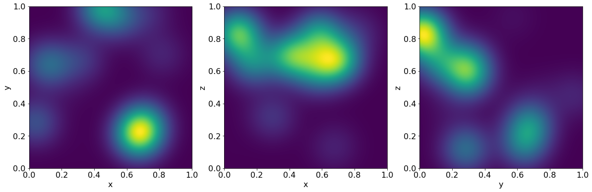
Let us test this implementation. We choose sources randomly in the unit box \([0, 1]^3\) and as targets we pick points in a grid along the three planes \(xy\), \(xz\) and \(zy\).
npoints = 400
nsources = 50

plot_grid = np.mgrid[0:1:npoints * 1j, 0:1:npoints * 1j]

targets_xy = np.vstack((plot_grid[0].ravel(),
                        plot_grid[1].ravel(),
                        np.zeros(plot_grid[0].size))).T
targets_xz = np.vstack((plot_grid[0].ravel(),
                        np.zeros(plot_grid[0].size),
                        plot_grid[1].ravel())).T
targets_yz = np.vstack((np.zeros(plot_grid[0].size),
                       plot_grid[0].ravel(),
                       plot_grid[1].ravel())).T

targets = np.vstack((targets_xy, targets_xz, targets_yz))

rand = np.random.RandomState(0)

# We are picking random sources

sources = rand.rand(nsources, 3)
Let us run the code and visualize the result using random weights.
%matplotlib inline
from matplotlib import pyplot as plt
from matplotlib.colors import LogNorm

plt.rcParams["font.size"] = 16

result = np.zeros(len(targets), dtype=np.float64)

weights = rand.rand(len(sources))

rbf_evaluation(sources, targets, weights, result)

def visualize(result, npoints):
    """A helper function for visualization"""

    result_xy = result[: npoints * npoints].reshape(npoints, npoints).T
    result_xz = result[npoints * npoints : 2 * npoints * npoints].reshape(npoints, npoints).T
    result_yz = result[2 * npoints * npoints:].reshape(npoints, npoints).T

    fig = plt.figure(figsize=(20, 20))

    ax = fig.add_subplot(1, 3, 1)
    im = ax.imshow(result_xy, extent=[0, 1, 0, 1], origin='lower')
    ax.set_xlabel('x')
    ax.set_ylabel('y')

    ax = fig.add_subplot(1, 3, 2)
    im = ax.imshow(result_xz, extent=[0, 1, 0, 1], origin='lower')
    ax.set_xlabel('x')
    ax.set_ylabel('z')

    ax = fig.add_subplot(1, 3, 3)
    im = ax.imshow(result_yz, extent=[0, 1, 0, 1], origin='lower')
    ax.set_xlabel('y')
    ax.set_ylabel('z')


visualize(result, npoints)

A parallel CUDA implementation#
We will now implement a CUDA version of this code. We assume that we have many more evaluation points than sources for the subsequent code. Each thread block will perform the evaluation for a small chunk of the target points and all source points. This strategy will not work if we have as many sources as there are targets.
import numba
from numba import cuda
import math


SX = 16
SY = nsources


@cuda.jit
def rbf_evaluation_cuda(sources, targets, weights, result):
    local_result = cuda.shared.array((SX, nsources), numba.float32)
    local_targets = cuda.shared.array((SX, 3), numba.float32)
    local_sources = cuda.shared.array((SY, 3), numba.float32)
    local_weights = cuda.shared.array(SY, numba.float32)

    tx = cuda.threadIdx.x
    ty = cuda.threadIdx.y

    px, py = cuda.grid(2)

    if px >= targets.shape[0]:
        return

    # At first we are loading all the targets into the shared memory
    # We use only the first column of threads to do this.

    if ty == 0:
        for index in range(3):
            local_targets[tx, index] = targets[px, index]

    # We are now loading all the sources and weights.
    # We only require the first row of threads to do this.

    if tx == 0:
        for index in range(3):
            local_sources[ty, index] = sources[py, index]
        local_weights[ty] = weights[ty]

    # Let us now sync all threads

    cuda.syncthreads()

    # Now compute the interactions

    squared_diff = numba.float32(0)

    for index in range(3):
        squared_diff += (local_targets[tx, index] - local_sources[ty, index])**2
    local_result[tx, ty] = math.exp(-squared_diff / ( numba.float32(2) * numba.float32(sigma)**2)) * local_weights[ty]

    cuda.syncthreads()

    # Now sum up all the local results

    if ty == 0:
        res = numba.float32(0)
        for index in range(nsources):
            res += local_result[tx, index]
        result[px] = res
nblocks = (targets.shape[0] + SX - 1) // SX
result = np.zeros(len(targets), dtype=np.float32)
rbf_evaluation_cuda[(nblocks, 1), (SX, SY)](sources.astype('float32'), targets.astype('float32'), weights.astype('float32'), result)
visualize(result, npoints)
Now let us benchmark the two versions against each other.
%timeit rbf_evaluation_cuda[(nblocks, 1), (SX, SY)](sources.astype('float32'), targets.astype('float32'), weights.astype('float32'), result)
5.61 ms ± 59.3 µs per loop (mean ± std. dev. of 7 runs, 100 loops each)
%timeit rbf_evaluation(sources, targets, weights, result)
204 ms ± 205 µs per loop (mean ± std. dev. of 7 runs, 10 loops each)
The Cuda implementation is on my laptop around 40 times faster than the parallel CPU implementation.